VisXplore is an R package for interactive data preprocessing and variable selection across mixed variable types. It computes pairwise correlations and associations for numeric, nominal (factor), and ordinal variables and visualizes the results as a network plot. It supports real-time data preprocessing and presents important information for variable selection.
VisXplore offers both a code-forward S3 API for use in R scripts and notebooks, and an optional Shiny app for interactive exploration.
Installation
You can install the development version of VisXplore from GitHub with:
# install.packages("devtools")
devtools::install_github("CU-Anschutz-GMWG/VisXplore")
Pairwise association
The core function pairwise_cor() computes a pairwise association matrix for all variables in a data frame. The association measure depends on the variable types involved:
| Variable pair | Measure |
|---|---|
| Numeric vs. numeric | Spearman rho |
| Factor vs. any | Pseudo R-squared (multinomial regression) |
| Ordinal vs. ordinal/numeric | Goodman-Kruskal gamma |
library(VisXplore)
result <- pairwise_cor(mtcars)
result
#> Pairwise associations for 11 variables (11 numeric)
#> 45 of 55 pairs significant at p < 0.05
#>
#> Variables: mpg, cyl, disp, hp, drat, wt, qsec, vs, am, gear, carb
Use summary() to view the full association matrix with significance stars:
summary(result)
#> Correlation/Association Matrix
#> Significance: **** p<0.0001, *** p<0.001, ** p<0.01, * p<0.05
#>
#>            cyl      disp        hp      drat        wt      qsec        vs
#> mpg  -0.91**** -0.91**** -0.89****  0.65**** -0.89****  0.47**    0.71****
#> cyl             0.93****   0.9**** -0.68****  0.86**** -0.57***  -0.81****
#> disp                      0.85**** -0.68****   0.9**** -0.46**   -0.72****
#> hp                                 -0.52**    0.77**** -0.67**** -0.75****
#> drat                                         -0.75****  0.09      0.45*
#> wt                                                     -0.23     -0.59***
#> qsec                                                              0.79****
#> vs
#> am
#> gear
#>             am      gear      carb
#> mpg   0.56***   0.54**   -0.66****
#> cyl  -0.52**   -0.56***   0.58***
#> disp -0.62***  -0.59***   0.54**
#> hp   -0.36*    -0.33      0.73****
#> drat  0.69****  0.74**** -0.13
#> wt   -0.74**** -0.68****   0.5**
#> qsec  -0.2     -0.15     -0.66****
#> vs    0.17      0.28     -0.63****
#> am              0.81**** -0.06
#> gear                      0.11
Use plot() to generate a network plot where node positions are derived from MDS on the dissimilarity matrix (1 - |association|), and edges represent associations above a minimum threshold:
plot(result, min_cor = 0.3)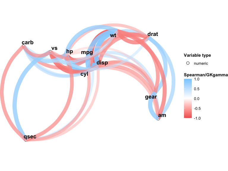
You can also customize the network plot directly with npc_mixed_cor():
npc_mixed_cor(result, min_cor = 0.5, show_signif = TRUE, label_size = 4)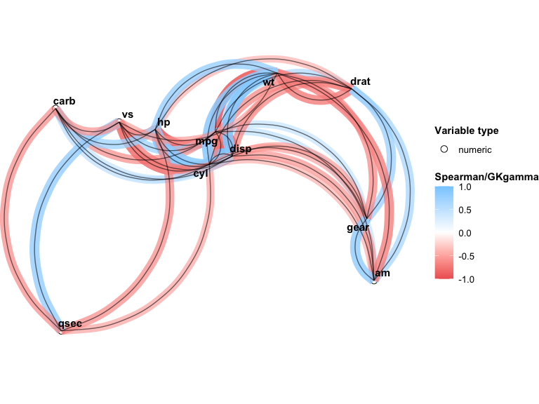
Mixed variable types
When your data includes factor or ordinal variables, specify the types explicitly:
types <- c("numeric", "factor", rep("numeric", 5), rep("factor", 2),
           rep("ordinal", 2))
result_mixed <- pairwise_cor(mtcars, types)
result_mixed
#> Pairwise associations for 11 variables (6 numeric, 3 factor, 2 ordinal)
#> 44 of 55 pairs significant at p < 0.05
#>
#> Variables: mpg, cyl, disp, hp, drat, wt, qsec, vs, am, gear, carb
Data quality checks
Use data_check() to identify empty or zero-variance columns before analysis:
df <- data.frame(x = rnorm(10), y = 1, z = NA)
data_check(df)
#> Warning: z missing for all observations
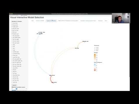
#> Warning: y with same value for all observationsInteractive Shiny app
For point-and-click exploration, launch the built-in Shiny app. It provides tabs for the network plot, variable distributions, correlation matrix, summary statistics, and data transformations:
VisXplore(mtcars)